Partitions in Apache Spark
One of the most important things to learn about Spark is that it's not magic. The framework still adheres to the rules of computer science. What I mean by this is that you can still do plenty of unoptimized workflows and see poor performance. Understanding how Spark works under the hood, from even a cursory level, can help in writing better Spark applications.
When writing Spark applications, I like to keep the following mental model. I am trying to understand something about the dataset I am working with, but I need to do it as efficiently as possible. This requires me to (1) scan over the fewest records possible, and (2) organize my scanning in such a way that produces the greatest efficiency. When considering distributed data, it's easy to neglect to consider either of these things. The performance and ergonomics of dealing with distributed data will largely be a function of how the data is distributed. In Spark, data is distributed in a master-worker fashion and when possible, all in-memory. The Resilient Distributed Data Set (RDD) is the data structure and API for dealing with distributed data. The RDD has some great features for performing large, distributed data operations. Under the hood of the RDD, data is stored into partitions. This chapter is intended to give you an introduction to partitions, what they are and some common gotchas when working with them.

A simple illustration of a Map Reduce operation. Data is split among three worker nodes, added together and returned to the master.
What is a partition?
My favorite way to think about a partition is with the following analogy. You work at a farmers market and your job is to keep track of how much fruit has been bought. At any time your boss might ask you to give them a count of how many strawberries are left, or how many apples have been bought. To begin each work day, you are given a crate of fruit that looks something like this:

An RDD represented as a crate of fruit.
Tracking how many of each type of fruit is in the box is a modern nightmare. You have to empty to box and count the fruit every time. There may be loose strawberries in the bottom or grapes and getting an accurate count is hard, especially after a large run of fruit. In order to make your job a bit easier, your boss gives you two additional crates. You split your large crate of fruit into two smaller crates. Now if you recruited someone to help keep track of the other box you now are twice as efficient, but the task is still not easy.
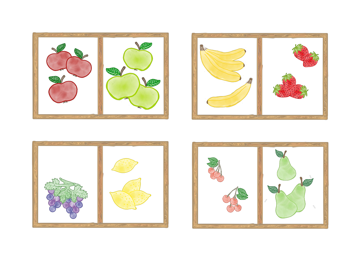
After some more consideration, you boss gives you 2 extra boxes and divider for each box. Now you separate fruit out by its type. Bananas with bananas, apples with apples and so on. You recruit 6 new people to work with you and getting a count of any fruit at any time is easy. Each person is in charge of well-organized fruit.

In this example, each box of fruit is a partition as part of an RDD. Some of the advantages of partitioning data, or separating it into organized chunks may be obvious already. Hopefully, through this chapter, we can solidify all of why it's valuable.
Group By
The way I described partitioning the fruit in the previous section is similar to grouping by type. You could imagine a query like this:
select * from fruit_box group by type;
The advantages of having the fruit partitioned in the way described are the same as the ones I listed above. We don't have to search through much data to get the answers we need and we can easily distribute the work of doing so. This way, we get the best performance and minimize the amount of time we spend moving data around. If we wanted to group to fruit by, say color, our partitions by fruit type wouldn’t be a helpful partition to have. We have red and green apples on the same partition, yet our red peaches are in a different box. In order to have an efficient group by, we would need to shuffle our data and re-order it.
In this case, our re-ordering would look something like this:

You'll notice we didn't need as many partitions but now we have mixed fruit again. Doing this would require a lot of work on our part, but much less since we already had the fruits sorted by type perviously. The process of reordering data into new partitions within an RDD is called shuffling.
Shuffle
Going back to the first example. Let's imagine we’re back in the place with the full crate of fruit:

The initial task of separating the fruit into their various partitions is the most time-consuming aspect of the entire operation. This is because the data is so out of order that we can’t say anything about it and it requires an immense amount of effort to get it organized. Doing this sorting and partitioning is called shuffling in Spark.

Workers sorting fruits into partititons
While workers tasks are isolated allowing them to do work quickly, they are not intelligent. Their main job is to just perform operations. They are not aware of other workers and they require the master to orchestrate any work between them. Shuffling is usually required when data order is not considered before performing an operation. For example, if you want a count of apples and your data is in the original color sorted state:

It’s much more time consuming to ask both partitions to figure out how many apples (red and green) there are. It would be ideal if we could put all the apples in the same partitions. Spark’s optimizations will find unoptimized partitions of data and shuttle it so that it can be organized properly for the algorithm you wish to be performed. It's much easier to load data from some source without consideration of how it's partitioned and try to perform operations. It's much more difficult to store data in formats (like ORC and Parquet) that make this consideration compared to csv files. While it is more work, the work quickly pays for itself as you can quickly get you data back to the partitions you want versus our original large crate.
Map
Suppose you wanted to count the bruises on all of the fruit in your crates and make a chart that looks like this:

A Map operation would be an appropriate way to accomplish this. As you can imagine, doing a map and ignoring the partitions is an expensive way of trying to accomplish this task. It would look something like this:

In general, Map is not a recommended way to execute this kind of operation. Spark is optimized to work on RDDs and partitions and not necessarily object by object.
Map Partitions

Map Partitions is a map operation over a partition. This allows you to (1) increase the amount of parallelism in a map operation and (2) optimize your map operation for partitions. I’ll solidify this point with our fruit example.
Supposed you’ve learned the easiest way to find bruises on each kind of fruit. So you can quickly find bruises on bananas or can tell from the color of the leaves on a strawberry that it has a bruise. You could allow different functions to operate and work their way through your partitions.

In my experience any Map operation I wanted to write I could rewrite it as a Map Partitions operation. One of the most common places where Map Partitions is used is in writing to a data store. By default, Spark operates in an append only mode. It wants to either add to an existing source or create a new source. Operations such as updating or deleting specific records are not supported with out of the box configurations. Often times, doing an update or upsert is necessary and using Map Partitions can help with that. Here is an example of how to do that:
Repartition
Returning to our example, suppose you added two more varieties of fruit to the daily offering. You get an extra crate and divider and create some new parititons:

Repartitioning this way has one advantage. It will distribute the data evenly across the partitions. This way, you have the same number of objects in each partition. It will require a shuffle and creation of an entirely new set of partitions. Additionally, just because they are evenly partitioned doesn't mean you won't have to shuffle on your next operation.
Using the Repartition is the nuclear option, but often necessary. In our case, there really isn't really a good alternative. If we know we want partitions by fruit type, this is what needs to happen. If we didn't care, we could just do a pure repartition and Spark would create an evenly distributed number of partitions.
Coalesce
Coalesce is like repartition, however, it does not require a shuffle. You can look at this as taking out one of the partitions in our example. You may or may not get evenly distributed partitions, but it may make sense to do this in a number of scenarios.
Consider my previous example of Map Partitions to write data to MySQL. You'll notice I used Coalesce there and reduced it to the number of machines I had available. I did this because of MySQL in that instance, preferred one connection per host. Since I had 16 cores on the workers, I could not open up 16 connections without running into trouble, I could share the connection with the 16 cores but I preferred to just use 4 machines and chunk the data that way for that example.
You have the freedom to make this decision, however, it is not a free operation. There is some cost to doing this but it is much less of a cost than repartitioning.
Windowing
Sometimes, the questions you have about data is more than a simple count. Suppose you want to know the average number of fruit sold or the average number sold by the day or by the hour? You could create a report that looked something like this:

Instead of keeping rotting fruit around, let's suppose we take our hand written data and append it to a parquet file every night. Now, we load that file into Spark. From here the partitions matter quite a bit. If we’re concerned about windowing over groups, time or both it's valuable to have the data partitioned that way. In this case, we should create partitions by day and fruit type.
Configurations
Through these examples, we have been able to successfully explore partitions in Spark and how they factor into writing good Spark applications. I didn’t talk much about how some of the basic configurations work around partitions. First, the default number of partitions are typically the number of cores available. In a distributed context this can either be the number of cores available. You can easily change this and add more or fewer partitions by using coalesce and adjusting the partitions.From a parallelism perspective, you should have more partitions than cores. This is simply from a divide-and-concur perspective.
Finally, a word on avoiding shuffles. You'll often hear about shuffles being the devil and to be avoided at all costs. I agree with this heuristic, however, I know in practice they are not 100% avoidable. I think the better caution is to reduce the number of shuffles using smart thinking around partitions.
Resources
One of the most helpful resources with partitions is the Spark UI. From this view, you can see how each of your operations relate to partitions and shuffling.

An example of the Spark UI.
If you have performance issues it’s most likely related to partitions, one way or another. Start here and work your way up the chain.
There are a great number of resources on partitions in Spark, here are 3 of my favorites. They are a bit heavier on the how to this post was much more focused on the conceptual underpinnings.